1.1 Observations

For some problems, the observations are represented directly, either as vectors in $\mathbb{R}^{m}$ or as elements on a manifold with $m$ degrees of freedom. For example, observations of points in an image are vectors in $\mathbb{R}^{2}$ ($m=2$). Observations of coordinate transformations in 3D are elements of $\mathrm{SE}(3)$ ($m=6$). In these cases, we refer to the collective observation as $\mathbf{z}\in\mathbf{Z}$. Often the collective observation is built by stacking up $M$ independent observations $\left\{ \mathbf{z}_{i}\in Z\right\}$:

$$\mathbf{Z} \equiv Z^{M}$$ (1)

$$\mathbf{z} \equiv \left(\begin{array}{c} \mathbf{z}_{1}\\ \vdots\\ \mathbf{z}_{M} \end{array}\right)$$ (2)

The observation model $\mathbf{h}(\mathbf{x})$ predicts the value of $\mathbf{z}$ given the state parameters:

$$\mathbf{h}:X\rightarrow\mathbf{Z}$$ (3)

The error vector $\mathbf{v}$ is then the difference (in a vector space) between the observations and the predictions, as a function of the parameters $\mathbf{x}$:

$$\mathbf{v}(\mathbf{x})\equiv\mathbf{z}\ominus\mathbf{h}(\mathbf{x})$$ (4)

When $\mathbf{z}$ is composed of independent observations $\left\{ \mathbf{z}_{i}\right\}$, we can also refer to the corresponding pieces of $\mathbf{v}$:

$$\mathbf{v}_{i}(\mathbf{x}) \equiv \mathbf{z}_{i}\ominus\mathbf{h}_{i}(\mathbf{x})$$ (5)

$$\mathbf{v}(\mathbf{x}) \equiv \left(\begin{array}{c} \mathbf{v}_{1}\\ \vdots\\ \mathbf{v}_{M} \end{array}\right)$$ (6)

The operator $\ominus$ yields a vector difference between two elements in $Z$:

$$\ominus:Z\times Z\rightarrow\mathbb{R}^{m}$$ (7)

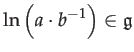
Its definition depends on that space. For observations in a vector space (e.g. image points), $\ominus$ is just the plain vector difference. For a Lie group $G$, and two elements $a,b\in G$, we can define

$$a\ominus b \equiv \ln\left(a\cdot b^{-1}\right)\in\mathfrak{g}$$ (8)

where $\mathfrak{g}$ is the Lie algebra vector space corresponding to $G$.

For some problems, the error function is easier to express directly, rather than as a difference between observation and model prediction. For instance, when estimating epipolar geometry, the errors are the distances between points in an image and their epipolar lines. Each distance $\mathbf{v}_{i}$ is a scalar ($m=1$), though the points themselves are 2-vectors and the predictions are lines. In such scenarios, we refer to the error vector $\mathbf{v}(\mathbf{x})$ without explicitly defining it in terms of $\mathbf{z}$ and $\mathbf{h}(\mathbf{x})$. Nonetheless, we still refer to the pieces $\mathbf{v}_{i}$ as observations.

We describe the uncertainty of $\mathbf{v}$ with a covariance matrix $\mathbf{R}$. In the case of Eq. :autorefequation4, $\mathbf{R}$ is typically just the covariance over $\mathbf{z}$ itself. Otherwise, $\mathbf{R}$ is computed by projecting uncertainties of the measured quantities into the space of the error $\mathbf{v}$. Again using the epipolar geometry example, the covariance of each point measurement is propagated through the distance-to-line function to yield variance over the epipolar error.

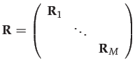
When the errors for each observation are independent, as is common in many optimizations, the matrix $\mathbf{R}$ is block diagonal with $M$ blocks, and we refer to the $i^{\mathrm{th}}$ block as $\mathbf{R}_{i}$:

$$\mathbf{R}=\left(\begin{array}{ccc} \mathbf{R}_{1}\\ & \ddots\\ & & \mathbf{R}_{M} \end{array}\right)$$ (9)