2 Gauss-Newton Method

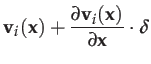
We approximate $\mathbf{v}_{i}$ as a function of $\mathbf{x}$ by a first-order Taylor expansion:

$\displaystyle \mathbf{v}_{i}\left(\mathbf{x}\oplus\boldsymbol{\delta}\right)$	$\displaystyle \approx$	$\displaystyle \mathbf{v}_{i}(\mathbf{x})+\dfrac{\partial\mathbf{v}_{i}(\mathbf{x})}{\partial\mathbf{x}}\cdot\boldsymbol{\delta}$
	$\displaystyle =$	$\displaystyle \mathbf{v}_{i}(\mathbf{x})-\mathbf{J}_{i}\cdot\boldsymbol{\delta}$

$\displaystyle \mathbf{v}\left(\mathbf{x}\oplus\boldsymbol{\delta}\right)\approx\mathbf{v}(\mathbf{x})-\mathbf{J}\cdot\boldsymbol{\delta}$

(22)

$\displaystyle L=\left(\mathbf{v}-\mathbf{J}\cdot\boldsymbol{\delta}\right)^{T}\cdot\mathbf{R}^{-1}\cdot\left(\mathbf{v}-\mathbf{J}\cdot\boldsymbol{\delta}\right)$

(23)

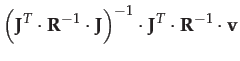
To minimize this residual, we differentiate with respect to $\boldsymbol{\delta}$ , set equal to zero, and solve for $\boldsymbol{\delta}$ :

$\displaystyle \dfrac{\partial L}{\partial\boldsymbol{\delta}}$	$\displaystyle =$	$\displaystyle -2\left(\mathbf{v}-\mathbf{J}\cdot\boldsymbol{\delta}\right)^{T}\cdot\mathbf{R}^{-1}\cdot\mathbf{J}$	(24)
$\displaystyle \mathbf{0}$	$\displaystyle =$	$\displaystyle \mathbf{v}^{T}\cdot\mathbf{R}^{-1}\cdot\mathbf{J}-\boldsymbol{\delta}^{T}\cdot\mathbf{J}^{T}\cdot\mathbf{R}^{-1}\cdot\mathbf{J}$	(25)
$\displaystyle \mathbf{v}^{T}\cdot\mathbf{R}^{-1}\cdot\mathbf{J}$	$\displaystyle =$	$\displaystyle \boldsymbol{\delta}^{T}\cdot\mathbf{J}^{T}\cdot\mathbf{R}^{-1}\cdot\mathbf{J}$	(26)
$\displaystyle \mathbf{J}^{T}\cdot\mathbf{R}^{-1}\cdot\mathbf{J}\cdot\boldsymbol{\delta}$	$\displaystyle =$	$\displaystyle \mathbf{J}^{T}\cdot\mathbf{R}^{-1}\cdot\mathbf{v}$	(27)
$\displaystyle \boldsymbol{\delta}$	$\displaystyle =$	$\displaystyle \left(\mathbf{J}^{T}\cdot\mathbf{R}^{-1}\cdot\mathbf{J}\right)^{-1}\cdot\mathbf{J}^{T}\cdot\mathbf{R}^{-1}\cdot\mathbf{v}$	(28)

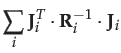
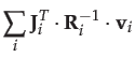
The Fisher information matrix $\left[\mathbf{J}^{T}\cdot\mathbf{R}^{-1}\cdot\mathbf{J}\right]$ is symmetric and positive definite, so the linear system can be efficiently solved with a Cholesky or $\mathrm{LDL}^{T}$ decomposition. Further, if the observations are independent, the information matrix and information vector are simply accumulated over the observations:

$\displaystyle \mathbf{J}^{T}\cdot\mathbf{R}^{-1}\cdot\mathbf{J}$	$\displaystyle =$	$\displaystyle \sum_{i}\mathbf{J}_{i}^{T}\cdot\mathbf{R}_{i}^{-1}\cdot\mathbf{J}_{i}$	(29)
$\displaystyle \mathbf{J}^{T}\cdot\mathbf{R}^{-1}\cdot\mathbf{v}$	$\displaystyle =$	$\displaystyle \sum_{i}\mathbf{J}_{i}^{T}\cdot\mathbf{R}_{i}^{-1}\cdot\mathbf{v}_{i}$	(30)

The update from Eq. :autorefequation31 is then applied by pertubring $\mathbf{x}$ by $\boldsymbol{\delta}$ :

$\displaystyle \mathbf{x}\leftarrow\mathbf{x}\oplus\boldsymbol{\delta}$

(31)

The whole process is iterated by evaluating $\mathbf{J}$ and $\mathbf{v}$ at the new parameters, recomputing $\boldsymbol{\delta}$ (Eq. :autorefequation28), and applying the update (Eq. :autorefequation31). The iteration continues until some convergence criterion is met, or the iteration count reaches a bound.

Note that upon convergence to a minimum of the residual, $\left(\mathbf{J}^{T}\cdot\mathbf{R}^{-1}\cdot\mathbf{J}\right)^{-1}$ (the inverse of the information matrix) is the Cramer-Rao lower bound for the covariance of the parameters.